Stata 101:
The Epidemiologist's Interface

Last Updated: 5 April 2026 • Environment: Stata 18 SE

Stata is one of the primary statistical environments used in epidemiology, public health, and health services research. It has a consistent command structure and a do-file system that makes reproducibility straightforward rather than optional. This guide introduces the interface, explains the do-file editor, and takes you through the first commands every epidemiologist needs to understand a dataset.

1. The Anatomy of Stata

Stata's layout is deliberately constrained. The interface uses four windows, each serving a fixed purpose. Learn what each one does and you will understand how Stata expects you to work.

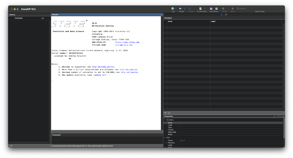
• The Results Window (Main Canvas): A scrolling log where Stata calculates your models, prints tables, and shows red error messages if your data is formatted incorrectly.
• The Command Window (Bottom): The terminal where you type isolated commands. This is useful to explore data quickly, but you should never use it for publishable analysis.
• The Variables Window (Top Right): A live list of every variable currently loaded in memory, its datatype, and attached labels.
• The Review / History Window (Left): A running ledger of every single action you have executed inside the session. If you accidentally run a command in the window, you can copy it from here.

2. The Golden Rule: The Do-File Editor

As an epidemiologist handling thousands of sensitive health records, reproducibility is the foundation of your work. We do not click buttons in dropdown menus.

Every single action, from loading the raw dataset to recoding categorical variables to running the final regression model, must be written sequentially in a Stata script. This is called a Do-File (.do).

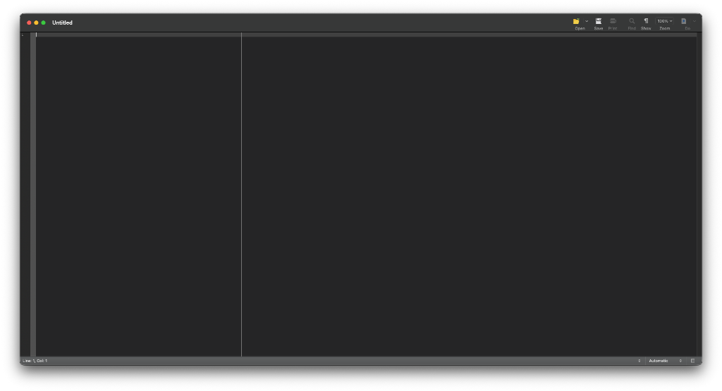
Do-File Editor

Open the Do-File editor by typing doedit in the command window. Write your code here. Highlight it and click the Execute (Do) button to run it. This saves your entire pipeline so colleagues can review it and peer reviewers can audit it.

3. Getting to Know Your Data

Before you run a single hazard ratio or logistic regression, you must intimately understand the shape of your cohort. Let us load a dataset directly into memory to understand the flow. Stata provides built-in health datasets for learning. We will use the bplong dataset, a hypothetical patient cohort tracking blood pressure over time.

Type this directly into your Do-File and execute it block by block:

* 1. Clear memory before starting
clear all

* 2. Load the built-in blood pressure dataset (sysuse grabs system datasets)
sysuse bplong

* 3. Describe the schema of the dataset
describe

The describe command tells you immediately how many observations exist and what variables are available. But it does not tell you if the data is messy. When loading real clinical data, your very first check should always be the codebook command.

* Get a granular breakdown of every variable, including missing values
codebook

codebook is arguably the most powerful exploratory tool in Stata. It prints a detailed report for every variable, showing the distinct unique values, the number of missing observations, and any text labels attached to numeric categories (like 1 = "Male", 2 = "Female").

Once you are satisfied your data is clean, you can generate summary statistics for continuous variables (like age or BMI) using the summarize command:

* Generate full summary statistics for the continuous blood pressure variable
summarize bp, detail

Alternatively, if you are looking at categorical epidemiological risk factors (like smoking status or Townsend deprivation quintiles), you need to look at cross-tabulations. We achieve this with tabulate (or simply tab for short):

* Generate a frequency table for patient sex
tabulate sex

* Generate a cross-tabulation of sex against age group, including row percentages
tabulate sex agegrp, row